Chapter 5 Spatial scale of control and mixing predicts dynamics of canine rabies

Abstract

Canine rabies is a devastating and preventable disease that causes a high burden of deaths globally each year, particularly in low-and-middle countries where investment in control is limited. Given the mounting evidence that elimination of these deaths is possible, the WHO has set a target to eliminate canine rabies deaths in humans by the year 2030. Mathematical models are a powerful tool to inform these efforts, but to date, efforts to develop robust modeling frameworks for domestic dog populations have been hampered by a lack of data, and inconsistencies between model results and observed dynamics. Here, we use a spatially rich, long-term dataset on canine rabies cases in the Serengeti District in Tanzania. Using parallel data on vaccination campaigns and the underlying spatial distribution of the domestic dog population, we use a simulation-based inference approach to fit our models to key spatiotemporal features of the data. We find that incorporating both the spatial scale of population mixing and the scale of control are key to recovering observed dynamics. We use these results to explore different vaccination scenarios, and find that high spatial coverage of vaccination campaigns is necessary to prevent outbreaks of canine rabies. Moving forward these results provide practical insights into control strategies and modeling methods, as well as shed light on key processes driving rabies transmission.

5.1 Introduction

Rabies is a devastating and fatal disease that causes an estimated 60,000 human deaths annually across the globe (Hampson et al. 2015). However, these deaths are preventable through post-exposure vaccination, which is highly effective at preventing death if administered promptly after exposure, and through vaccination of domestic dogs, which with sufficient coverage can interrupt transmission and lead to elimination (Lankester et al. 2014). The World Health Organization and its partners have set a goal to eliminate deaths due to canine-mediated rabies by the year 2030 through a combination of these interventions (Abela-Ridder et al. 2016).

While there is a rich history of modeling wildlife rabies transmission dynamics, the body of work for canine rabies is much sparser. Critically, traditional models of wildlife rabies dynamics fail to capture patterns of incidence observed in endemic and epidemic scenarios for dog rabies (i.e. low and persistent endemic incidence without substantial depletion of the host population). However, we have a strong understanding of rabies epidemiology and biology: transmission does not appear to scale with dog densities evidenced by consistent \(R_{0}\) estimates between 1 - 2 across a range of settings; the infectious period is short and infection is almost invariably fatal; and key epidemiological parameters such as the dispersal kernel and the incubation period are characterized by a long tail. While R0 estimates are consistent and low, there is considerable heterogeneity in transmission with many infectious dogs biting no others, while some may bite upwards of 20 - 50 others (Rajeev, Metcalf, and Hampson 2020).

While the epidemiological backbone of rabies is clear, there is little data on disease dynamics in domestic dogs with which to confront models (Scott et al. 2017). In fact, most modeling studies of canine rabies are simulation based, with few studies actually fitting models to data (Rajeev, Metcalf, and Hampson 2020). This is largely due to poor surveillance (likely substantially less than 5% of cases are detected annually in endemic settings(Sunny E. Townsend et al. 2013)), but given the epidemiological features of rabies combined with low detection rates, inference can be challenging. Rabies outbreaks are highly stochastic and likely driven by heterogeneities and rare events. Therefore traditional inference methods based on times series data alone are likely to fail when confronted with the noisy reality of rabies data.

Recent advances in simulation based inference have facilitated fitting to data from highly stochastic and noisy systems using more complex models with analytically intractable likelihoods (Funk and King 2020; Hazelbag et al. 2020). One such method is Approximate Bayesian Computation, with fits to features of the data rather than each individual observation (Hazelbag et al. 2020). These methods are useful tools for model comparison, and present a way forward to assess what level of complexity is needed in models to predict observed dynamics.

Here we use a uniquely comprehensive long-term dataset on canine rabies cases in space and time across the Serengeti District in Tanzania, where ongoing vaccination campaigns have shaped dynamics over the past twenty years. We build on recent work that highlights the role of spatial structure in mixing (Mancy et al., n.d.), simplifying the model, extending it to consider different movement scenarios, and comparing models at the scale of population mixing (~ 1 km) vs. at the scale of control (village scale). Coupled with data on vaccination and the spatial distribution of the dog population, we build an individual-based spatially explicit model, and using a simulation-based inference approach, fit it to key spatiotemporal features of the observed data to identify models that best fit our data and generate realistic dynamics in endemic situations. Finally, we simulate vaccination campaigns and control strategies based on our findings to inform control efforts.

5.2 Methods

5.2.1 Study area

The Serengeti District in Tanzania is approximately 2000 km² in area and is comprised of of multi-ethnic agropastoralist communities (estimated human population of 2.49^{5} at the time of the last census in 2012) with high dog ownership (estimated human-to-dog ratios ranging from 3 to 9). Rabies has been endemically circulating in the district, with documented outbreaks reported as early as the 1950s (Brunker et al. 2015), and rabies vaccination campaigns have been ongoing in the district since the early 1990s. Through multi-institutional partnerships with the Tanzanian government and vaccine manufacturers, these have expanded into a large scale control program.

Since 2002, a long-term contact tracing study of canine rabies and domestic dogs has been ongoing in the district (Hampson et al. 2009b), with data collected on clinical and laboratory diagnosed cases of animal rabies, as well as vaccination and dog ownership data. Here we use three key datasets from this study system:

1. Case histories of clinical and laboratory diagnosed dog rabies cases between 2002 - 2020 (N = 3179 observations with and approximate date of symptom onset and GPS location (5.1A and B).

2. 3. A full household and dog census of the district conducted between 2009 - 2014, with the spatial location of households, the number of people and of adult dogs and puppies in each household, and their vaccination status (5.1C).

3. A full household and dog census of the district conducted between 2009 - 2014, with the spatial location of households, the number of adult dogs and puppies in each household, the number of individuals in these households, and dog vaccination status (5.1D).

We also used census data on human population sizes from the 2002 and 2012 national census in Tanzania to estimate population growth over the district. Village (i.e. administrative level 3) boundaries for the district were constructed using the distribution of household locations belonging to each village from the dog census data (5.1D, (Mancy et al., n.d.)).

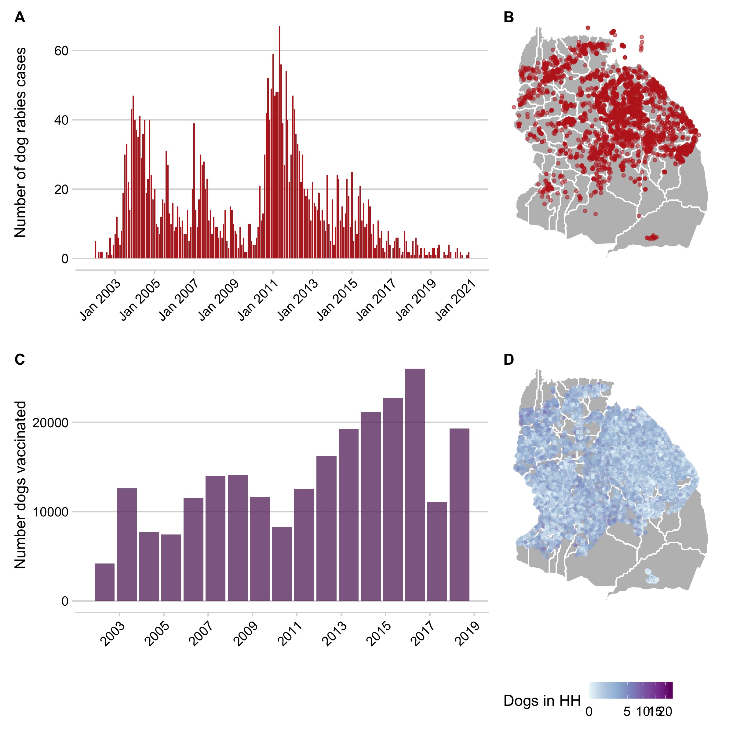
Figure 5.1: Datasets used in the analyses. A) Shows the time series of monthly rabies cases in domestic dogs and B) shows their spatial distribution across the district. C) The annual number of dogs vaccinated each year during mass campaigns. D) The location of household census data with colors showing the number of dogs owned per household. Polygons delineate village boundaries in the district.

5.2.2 A spatially-explicit, individual-based model of rabies transmission

We developed a discrete-time, individual-based, Susceptible-Exposed-Infectious-Vaccinated transmission model to simulate rabies dynamics in the domestic dog population. Transmission occurs at the individual level with secondary cases drawn from a right censored negative binomial distribution with mean \(R_{0}\) and dispersion parameter \(k\) (to capture heterogeneity, but constrained so that secondary cases from a single individual do not exceed 100 cases, a realistic range of transmission potential). Movement of infectious individuals occurs in continuous space, with distances either drawn as a dispersal distance (log normal distribution, i.e. case movements are all drawn in reference to the progenitor location) or as a random walk with a Weibull step length distribution, (i.e. case movements are sequential). The timing of when a dog becomes infectious after exposure is drawn from a lognormal serial interval distribution (the infectious period + the incubation period). Previous work has shown the importance of introductions of rabies cases from outside the district in maintaining transmission within the district (Mancy et al., n.d.). We use two approaches to simulate introductions:

1. Using inferred locations of introductions from transmission tree reconstruction between 2002 - 2015 to explicitly seed transmission chains
2. Drawing the number of weekly introductions as a poisson distributed variable (\(\iota\)) and randomly seeding them in space

Demographic processes occur sequentially and are aggregated to the spatial scale being modeled: new dogs are born according to village level birth rates; dogs die at a fixed rate across the district, and finally vaccination occurs. Vaccinations are allocated from the village level to the spatial scale being modeled, allocated by population size in a given location, and we assume that surviving vaccinated dogs are re-vaccinated in subsequent campaigns, giving a conservative estimate of vaccination. To get initial dog population sizes in each location, we estimate human:dog ratios from the dog census data, and apply them to human population estimates from national census data at the start of our simulation period (2002). We allocate them spatially according to the distribution of households and dogs from the census data. To get village level growth rates, we estimate human population growth between 2002 - 2012 from the national census data at the village level and assume that dog populations grow at that same rate (and assume a fixed death rate, Table 5.1 (Czupryna et al. 2016)). We do not apply demographic transitions to exposed or infectious individuals (i.e. they only move out of their classes when moving from exposed to infectious or infectious to removed).

We use a weekly time step to aggregate both demographic and transmission events (i.e. infectious dogs in location x at week t all compete for the same contacts) and explore different scales of spatial mixing: at an 1 km² resolution and at the village scale (in UTM Zone 36S such that distances between grid cells are as close to 1 km as possible). Table 5.1 lists all parameters and their sources. In addition to comparing mixing at the village and 1 km scales, we also explore how further constraining movement of rabid dogs impacts model inference. At the baseline, we do not constrain movements of rabid dogs: that is rabid dog movements to locations outside of the district or to inhabited patches will result in a failed transmission event. We compare this baseline (which we refer to hereafter as the no limits model) with a model that restrict movements to only inhabited patches (i.e. populated patches at the beginning of the simulation, the patch limits model), and finally a model that restricts movement to both uninhabited patches and to the district (the full limits model). For the constrained models, we do not resample individual movements that fail as this could potentially skew the underlying parameter distance distribution (for example, if resampling happens often enough, this can shift both the average and skew of the distribution). Instead, for each movement we draw distances, find grid cells within that distance, and sample movement to valid locations given the model constraints. We assume that infection is completely fatal, and infectious individuals are removed at the end of the weekly timestep during which they became infectious. Finally, to account for imperfect case detection we use a monthly beta binomial detection probability (Table 5.1).

Table 5.1: Table of parameter inputs and sources.

Input (units)	Distribution	Source
Secondary case distribution (number of dogs)	Right censored negative binomial distribution with mean = \(R_{0}\) and dispersion parameter \(k\)	\(R_{0}\) and \(k\) are estimated, prior centered around estimates from Hampson et al. (2009b)
Weekly rate of introductions	Poisson distribution	Estimated
Serial interval distribution (days)	Lognormal distribution with mean = 2.95, and sd = 0.86, for a mean interval of approximately 27 days	Mancy et al. (n.d.)
Dispersal kernel (meters)	Lognormal distribution with mean = 5.58, and sd = 1.79, for a mean dispersal length of approximately 1483 meters	Mancy et al. (n.d.)
Step length distribution (meters)	Convolved Weibull distribution with shape = 1.12, and scale = 491.1, for a mean step length of approximately 428.35 meters	Mancy et al. (n.d.)
Detection probability (monthly)	Beta binomial distribution with \(\beta\) = 8.9, \(\alpha\) = 80.1, for a mean monthly detection probability of approximately 0.9	Mancy et al. (n.d.)
Annual death rate (dogs/yr)	1/25.8 yrs	Czupryna et al. (2016)
Rate of waning vaccine immunity (dogs/yr)	1/3 yrs	Hampson et al. (2009b)

5.2.3 Model selection & parameter estimation

We use Random Forest Approximate Bayesian Computation (RF-ABC) implemented in the R package abcrf (Pudlo et al. 2015; Raynal et al. 2018) to perform model selection and parameter inference. We estimate three parameters: \(R_{0}\) (the mean of the secondary case distribution), \(k\) (the dispersion parameter of the secondary case distribution), and \(\iota\) (the mean weekly number of introductions of rabies cases from outside of the district). We use strong priors based on previous analyses of part of this dataset (Table 5.1)(Hampson et al. 2009b). RF-ABC can be used to evaluate both models and potential summary statistics (i.e. key features of the data that the model should capture). Table 5.2 lists the candidate summary statistics we used for model selection and parameter estimation, encompassing temporal, spatial, and spatiotemporal metrics of the data. RF-ABC ranks each of these parameters by their importance (i.e. Gini importance, specifically how frequently a variable is used for node classification and broadly a relative measure of the discriminative value a statistic has for the classification problem) in predicting a given parameter or in differentiating models. For both model selection and parameter estimation, we generate N = 1e5 simulated sets of summary statistics. To manage computational resources, we stop any simulations where the host population has declined to greater than 15% of the starting population, as these simulations generally lead to extinction of domestic dogs and represent unlikely scenarios. We include these simulations in the dataset, but calculate summary statistics only including the data before the simulation was stopped.

We use the default parameter of 500 trees in the random forest for estimation, and also perform a sensitivity analysis with subsets of the full dataset (subsampling to 75% of simulated dataset) to assess whether estimates are stable. We use prior error rates (the error rate of model classification on simulated datasets withheld from each of the classification trees, i.e. out-of-bag simulations) for model selection to assess the stability of model estimates to the number of simulated datasets and the number of trees in the Random Forest (Raynal et al. 2018). RF-ABC does not allow for joint parameter estimation, however, we approximate joint posteriors by including parameter sets where all estimated parameters were accepted (i.e. all values were assigned non-zero weights by the random forest classification). We also tested the ability of models to see recovered known parameter estimates using the model to predict out-of-sample simulated datasets across the parameter priors.

We perform model selection for models across all combinations and estimate their posterior probabilities (i.e. given our observed data, the proportion of trees in our RF model that predicted a given model). We then simulate from the estimated posterior distributions (N = 1000) and compare this to our observed data. We score simulations using the continuous ranked probability score (Jordan, Krüger, and Lerch 2019), and for each simulation of the monthly time series, we also generate centrality scores (i.e. how representative is a given simulation of the ensemble, (Juul et al. 2020)) and also the root mean squared error (RMSE) against the observed monthly cases. We also simulate an endemic scenario with no vaccination to see if the models can generate realistic dynamics in this context.

Table 5.2: Summary statistics used for fitting in Random Forest ABC.

Summary statistic	Description	Type
Max I	Maximum monthly number of cases	Temporal
Median I	Median monthly number of cases	Temporal
Mean I	Mean monthly number of cases	Temporal
Temporal KB	Kullback-Leibler Divergence between observed and simulated distribution of cases temporally	Temporal
Spatial KB	Kullback-Leibler Divergence between observed and simulated distribution of cases spatially	Spatial
Mean distance 4 weeks	Mean distance between cases within an 4 week window	Spatiotemporal
Mean distance 8 weeks	Mean distance between cases within an 8 week window	Spatiotemporal
Mean distance 4 weeks normalized	Mean distances of cases within an 4 week window, normalized by the average distance between all cases	Spatiotemporal
Mean distance 8 weeks normalized	Mean distances of cases within an 8 week window, normalized by the average distance between all cases	Spatiotemporal
Spatial RMSE	Root mean squared error between the observed vs. simulated density of case locations	Spatial
Spatial loss	Loss value of the absolute difference between observed and simulated cases locations	Spatial
Temporal RMSE	Root mean squared error between the observed vs. simulated numbers of monthly cases	Spatial
Temporal loss	Loss value of the absolute difference between observed and simulated monthly cases	Temporal
Mean distance all cases	Average distance between all cases	Spatial
ACF Monthly 1-6	Autocorrelation values for monthly time series at 1 - 6 month lag	Temporal
ACF Weekly 1-10	Autocorrelation values for weekly time series at 1 - 10 week lag	Temporal

5.2.4 Assessing simulated vaccination campaigns impact on transmission

To explore how spatial heterogeneities in vaccination coverage could drive outbreak risk, using the model with the highest posterior probability given our observed data (our ‘best’ model), we simulate across a range of campaign scenarios. We vary both the level of coverage achieved during annual campaigns (campaign coverage), and the proportion of villages which are vaccinated during campaigns (spatial coverage), and use our posterior estimates to simulate transmission dynamics. We simulate these campaigns (N = 100 simulations per combination) with random villages being vaccinated with probability x in each year. We simulate a five year endemic burn-in period, and then simulate annual campaigns over ten years. In the last five year period of the simulation, we calculate summary statistics that capture key metrics of control success such as peak and mean incidence, chain size and length, and weeks where transmission exceeds the 95th% of the mean incidence of introduced cases only. We also calculate a connectivity based summary statistic at the village level (c) which equals the sum of squares of the component size of the village graph, where villages are connected if they are adjacent and if coverage at that time step exceeds a threshold (the campaign coverage for a given simulation).

5.2.5 Assessing the impact of additional interventions on transmission and outbreak probabilities.

Using our best model, we explore how additional interventions implemented alongside vaccination campaigns affect outbreak probabilities and transmission. We simulate approximations of two different interventions in combination with the random village campaigns as described above: 1) ‘Chopping the tail’ of the secondary case distribution (Kain et al. 2020), where we decrease the censoring value as vaccination increases, to approximate how enhanced surveillance and isolation/quarantine/removal of rabid dogs can improve control outcomes 2) Reducing introductions as coverage increases, i.e. approximating coordination of vaccination campaigns across larger spatial scales

Fig 5.18 shows the simulated reductions in introduction rates and maximum allowed secondary cases given district level coverage..

5.2.6 Data and ethics statement

The data used in these analyses are part of a long term research project in the Serengeti District approved through the University of Glasgow Ethics Board and by the Tanzania Commission for Science and Technology, and National Institute for Medical Research. Anonymized data and code are available at github.com/mrajeev08/dynamicSD (to be archived on Zenodo and made public upon article submission) and the underlying simulation model is available here (github.com/mrajeev08/simrabid). All analyses were done using R (R Core Team 2020) and the following key packages: abcrf, ranger, data.table, sf, raster, and foreach, (Pebesma 2021; Dowle and Srinivasan 2020; Wright, Wager, and Probst 2020; Hijmans 2020; Revolution Analytics and Weston, n.d.; Pudlo et al. 2015).

5.3 Results

5.3.1 The scale of mixing and specification of introductions differentiate models.

Model predictions largely varied across two axes: whether introductions were estimated or fixed within the model and the scale of mixing (a 1km² scale vs. the village scale). The models with kernel based movement and with estimated introduction rates were ranked highest at both scales, Whether movement was constrained (patch limits or full limits model) did not seem to impact model selection (Fig 5.7). Summary statistics that best differentiated the models encompassed both spatial and temporal summary statistics, and the linear-discriminant analysis axes (LDAs, decompositions of our summary statistics) generated by the RF ABC model (Fig 5.2B). These results were robust to subsampling the datasets (Fig 5.8) and out-of-bag prior error rates were relatively stable with inclusion of additional trees in the random forest model (Fig 5.9). However, broadly, all the models and priors failed to consistently recapture the major components of the summary statistics (Fig 5.2A) or clearly differentiate between models within scales (a high prior error rate, with datasets withheld from the classification model misclassified approximately rround(prior_err_rate, 2)*100)`% of the time) (Fig 5.7).

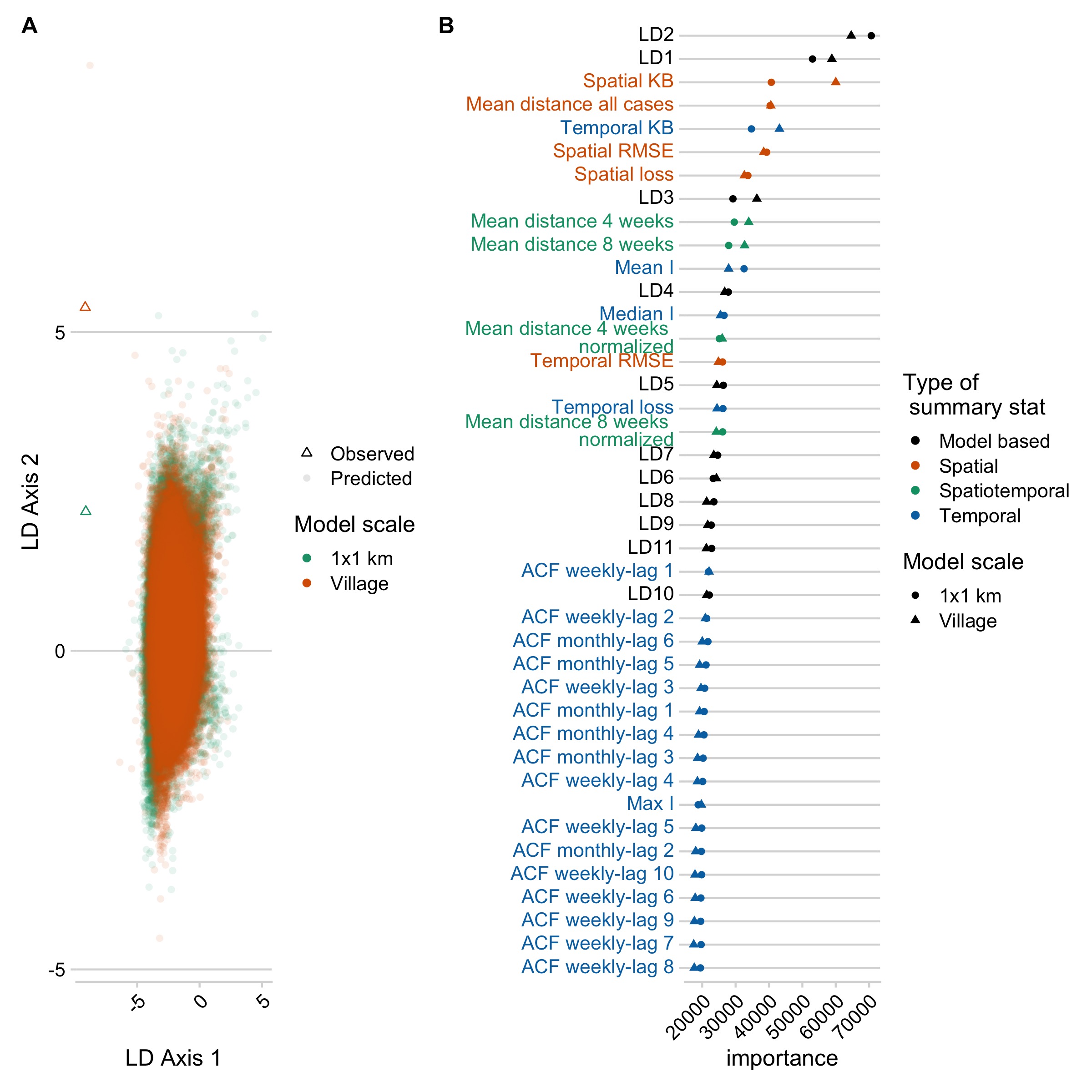
Figure 5.2: Model selection using RF ABC. A) The two major LDA axes generated by the random forest model for the best model at the village and 1 km scale, with the LDA values predicted for the observed data shown as triangles. B) The importance ranking of each variable in discriminating between models.

5.3.2 Capturing the spatial scale of vaccination and of mixing is key to recovering the observed trajectory of rabies in the Serengeti District.

We estimated three parameters: \(R_{0}\), k, and \(\iota\) (for models estimating introductions) using these same models and summary statistics. \(R_{0}\) was best predicted by temporal summary statistics, while k and \(\iota\) were predicted by spatial and spatiotemporal summary statistics (Fig 5.3, Fig 5.10). Estimates of \(R_{0}\) were consistent and identifiable across the models and robust to subsampling simulations (Fig 5.12), but varied significantly across scales and introduction scenarios (Fig 5.11). When comparing posterior estimates for the best models at each scale, \(R_{0}\) estimates were lower in models at the village scale when compared to the 1 km scale (Fig 5.4, Table 5.3). Estimates of k and \(\iota\) were more diffuse, and when filtering to parameter sets that had been accepted jointly (i.e. had non-zero weights for all three parameters), estimates of the introduction rate became sharper, while k became bimodal/skewed (Fig 5.11). When we tested the best models at each scale to see whether simulated datasets which were not included in the model fitting could be recovered, we found that \(R_{0}\) and \(\iota\) could be recovered robustly across our prior range, but k was largely unidentifiable (5.13).

Table 5.3: Priors and independent and joint posterior parameter estimates (mean with 95% quantiles in parentheses) for the best model at each scale.

Scale	Parameter	Prior	Independent posterior	Joint posterior
1x1 km	\(R_{0}\)	1.13 (0.75 - 1.63)	1.14 (0.99 - 1.28)	1.13 (0.97 - 1.27)
1x1 km	\(k\)	1.45 (0.48 - 3.44)	3.04 (0.84 - 7.5)	4.12 (1.26 - 7.16)
1x1 km	\(iota\)	1.13 (0.37 - 2.67)	1.8 (0.81 - 4.63)	1.31 (0.85 - 2.14)
Village	\(R_{0}\)	1.13 (0.75 - 1.63)	1.02 (0.91 - 1.13)	1.03 (0.92 - 1.11)
Village	\(k\)	1.46 (0.48 - 3.44)	3.43 (0.97 - 8.13)	4.16 (0.78 - 6.28)
Village	\(iota\)	1.13 (0.37 - 2.67)	2.16 (1.03 - 4.19)	1.59 (1 - 2.26)

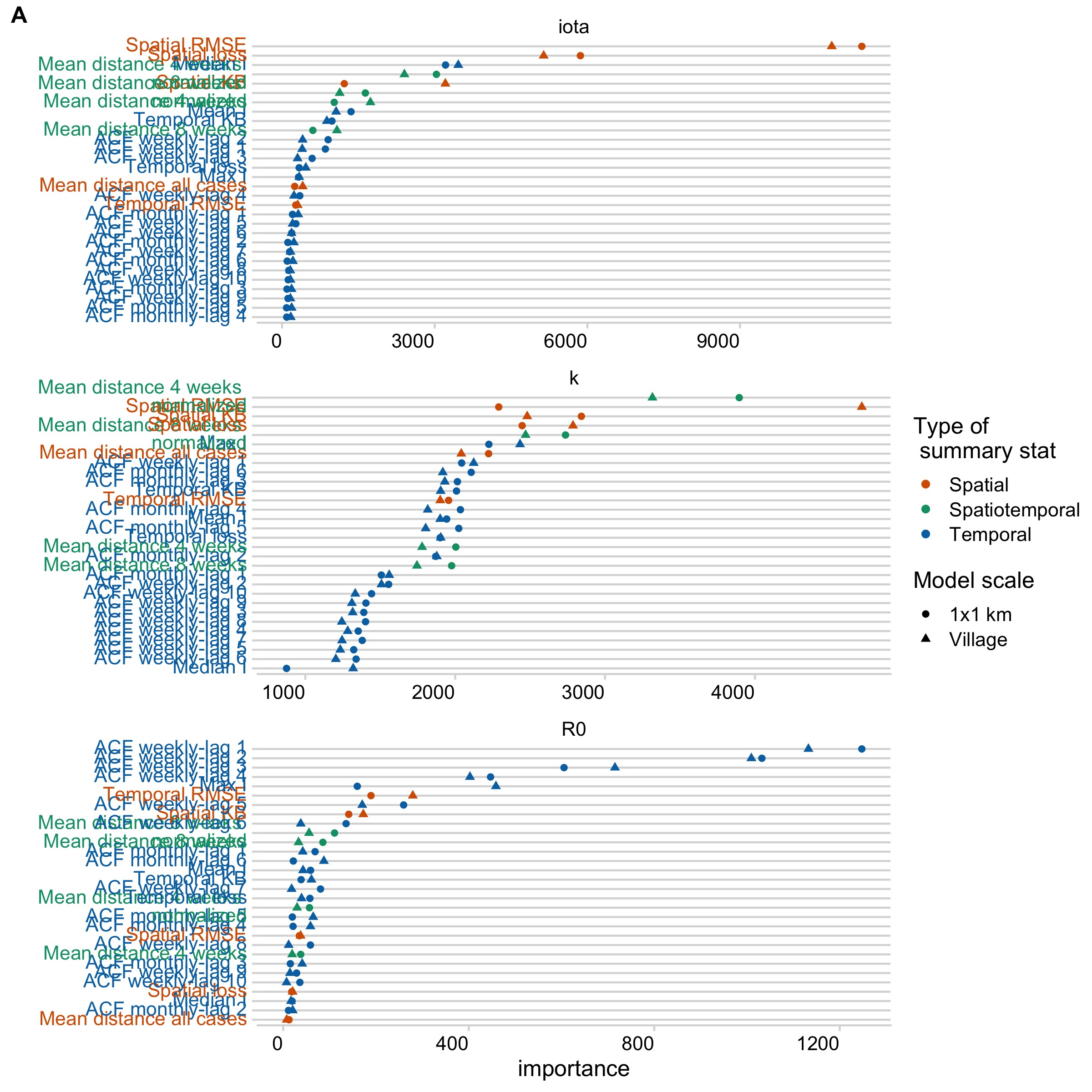
Figure 5.3: Ranking of summary statistics for importance in predicting each parameter. Summary statistics are colored by the type of statistic (either spatial, temporal, or spatial temporal). Results are shown for the best fitting model at the village and 1 km scale.

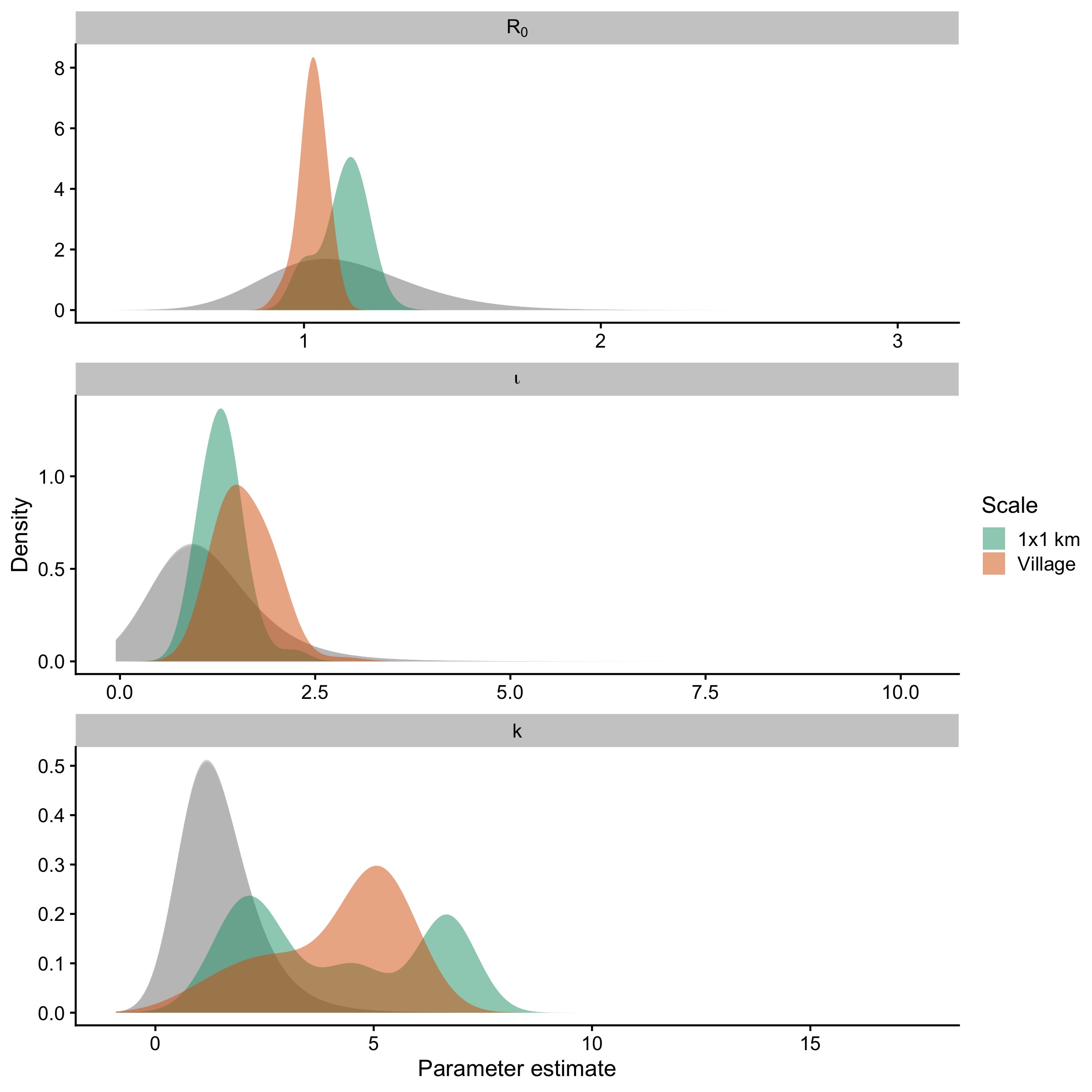
Figure 5.4: Joint posterior estimates compared to prior for the best fitting model at the village and 1 km scale for the three parameters, with prior density in grey.

When simulating the data from the posteriors, the models ranked highest by the RF ABC method estimates result in simulations closest to the data observed (Fig 5.5, Fig 5.14). Sampling from the joint parameter sets also improved fits to the data (Fig 5.15, Fig 5.16). At both the village and 1 km scale, simulations encompass the trajectory of cases we observed. However, the village scale model fails to capture stable dynamics in an endemic scenario with no vaccination, with transmission resulting in significant declines in the host population, while models at the 1km scale generate stable endemic incidence without depleting the host population (Fig 5.17).

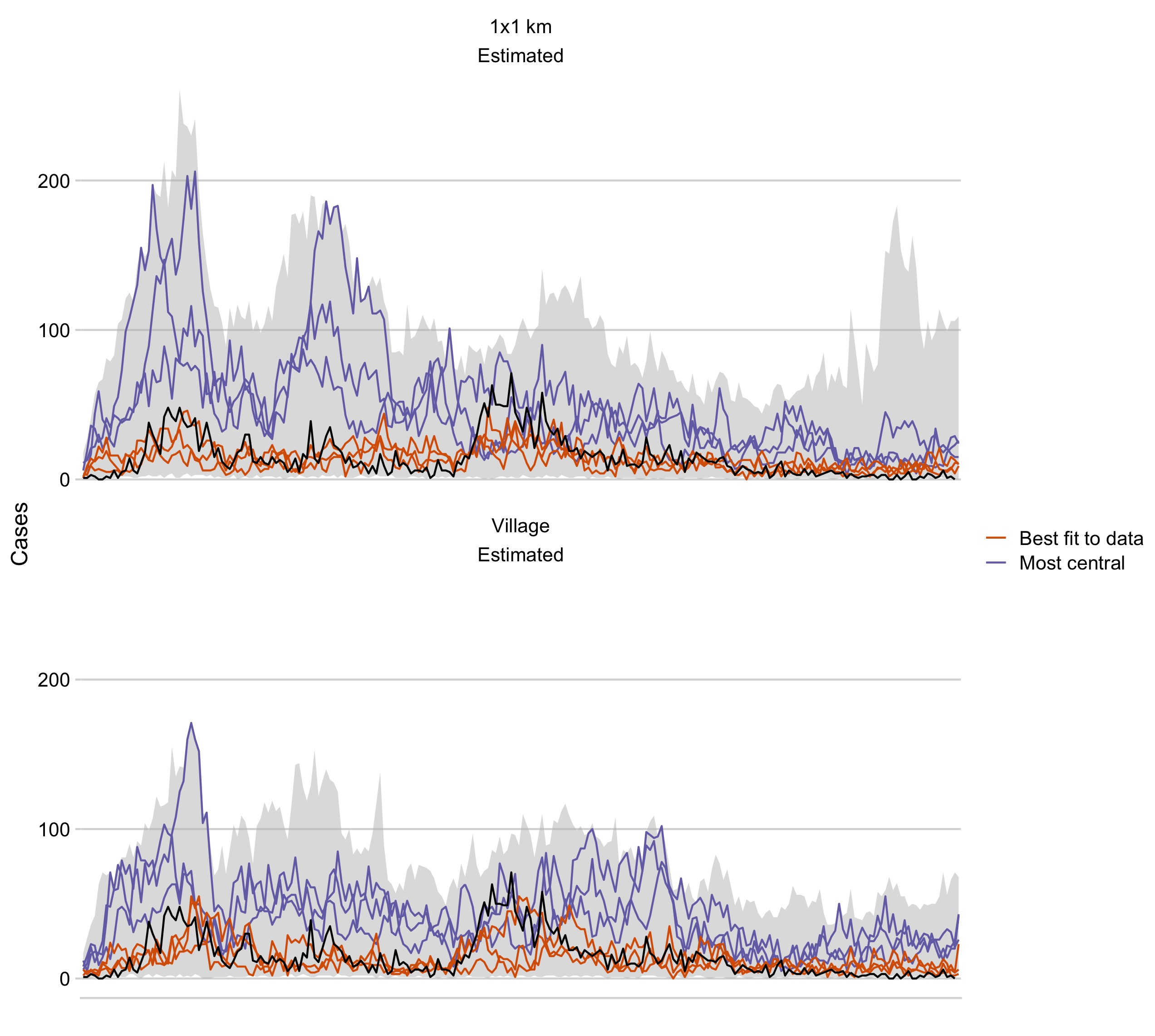
Figure 5.5: Simulations from the joint posterior distributions of the best fitting model. The grey envelope shows the range of simulations, and the black line is the time series of observed monthly cases. The orange lines show the top three simulations that best fit the data (lowest RMSE) and the purple lines show the top three simulations that have the highest centrality score.

5.3.3 Spatial coverage of vaccination predicts control outcomes and interventions that target key features of transmission improve these outcomes.

We find that control outcomes are strongly predicted by both campaign (i.e. the coverage level achieved by a village campaign) and spatial coverage (the proportion of villages covered by a campaign)(Fig 5.19). We find that campaigns that achieve an annual campaign coverage of 80% of the population at the village scale and a spatial coverage of 80% of villages vaccinated are most likely to prevent outbreaks of canine rabies (defined as greater than 4 months with weekly cases greater than the 95% of the average of the introduced cases) (Fig 5.6). These broadly track with other metrics of control outcomes as well, such as the average peak size and length of transmission chains, and mean and peak incidence (Fig 5.19). In general, both spatial and campaign coverage are more predictive of peak rather than average metrics (Fig 5.19). Connectivity of vaccinated villages varies the most at intermediate spatial coverage, and this metric also broadly predicts control outcomes within a given campaign scenario (Fig 5.22).

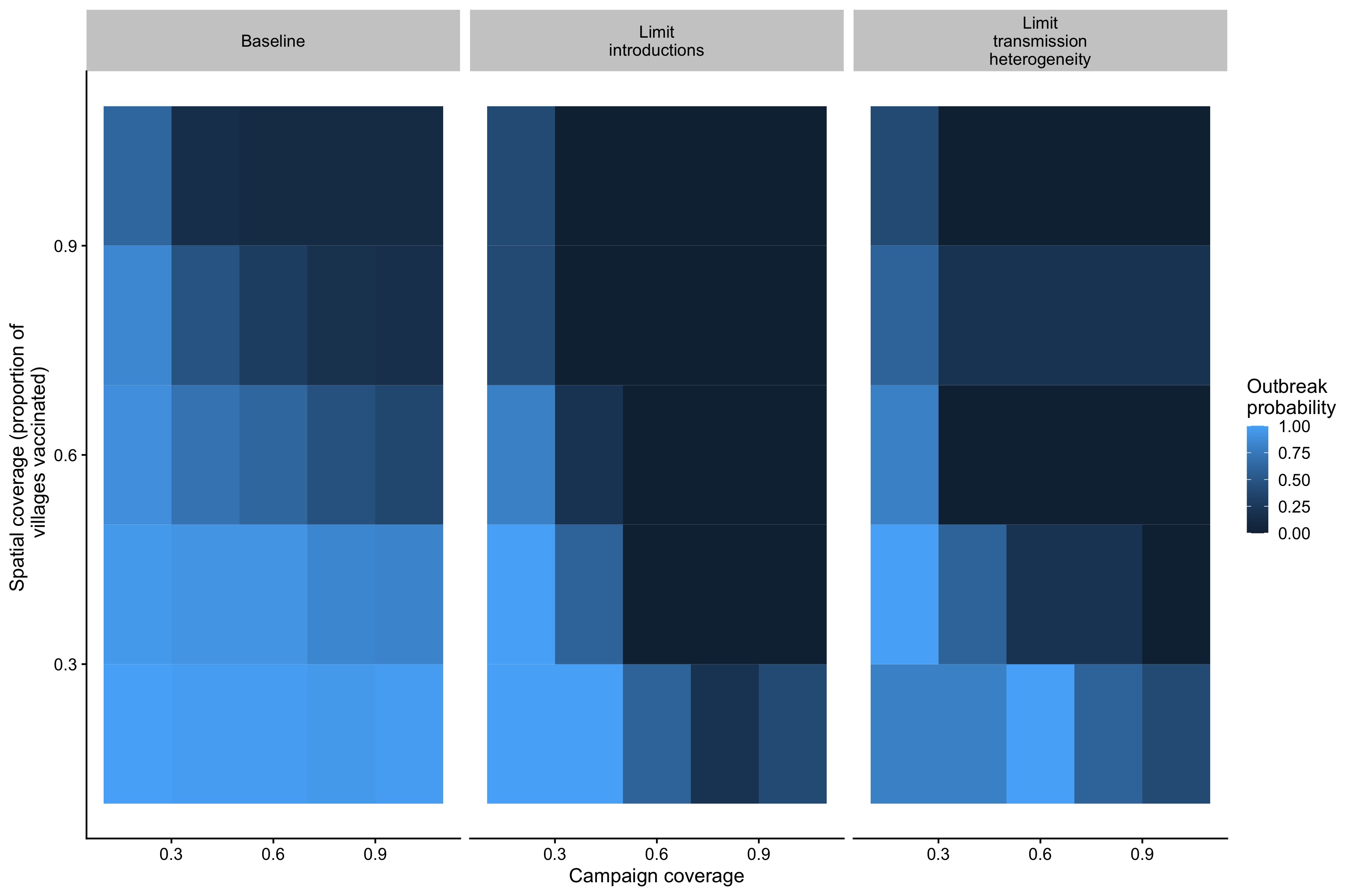
Figure 5.6: Outbreak probabilities (defined here as whether the number of consecutive weeks with cases above the 95th% of the incursion rate exceeding 16 weeks) in relation to a range of campaign coverage and spatial coverage under the baseline scenario and with the additional limits on transmission heterogeneity and introductions.

Two additional control strategies, one increasingly censoring transmission as coverage increases, approximating control strategies such as tracing and quarantine, and the second reducing the introduction rate as coverage is increased, approximating coordinated control efforts across larger geographic scales, also greatly improve control outcomes (Figs 5.21 and 5.20). In particular, reducing the introduction rate shifts both the spatial coverage and campaign coverage required to limit outbreaks (Fig 5.6).

5.4 Discussion

Overall, we find that accounting for both the spatial scale of vaccination and of mixing is critical to capturing the observed dynamics of canine rabies in the Serengeti District. Confirming previous work, we show that modeling transmission at the scale of dispersal (~ 1km) is key to capturing stable endemic dynamics and also result in parameter estimates closest to empirical estimates from individual scale data. We also found that introductions of cases from outside the district are crucial to the maintenance of transmission. Importantly, spatial and spatiotemporal features of the data were key to differentiating between models and identifying parameter estimates, and the time series statistics of the data were generally the least predictive of model separation or parameter estimates. We find that high spatial coverage of vaccination campaigns is key to predicting control outcomes, even at a coarse administrative level. Here, we define \(R_{0}\) as the mean of the offspring distribution, but not as a critical threshold for persistence. Our results suggest that moving away from simplistic herd immunity thresholds to more nuanced targets, (i.e. 70% of dogs in at least 70% of villages), may better predict control outcomes. In addition, given the importance of transmission heterogeneity and introductions in transmission, control measures targeted at these key features, i.e. coordinating control across larger geographic scales, could compound the dividends gained through vaccination alone.

We use a uniquely comprehensive data set in both temporal and spatial scope in our analysis. This data allow us to pin down key features and expectations of rabies transmission, and the vaccination and population data provide a lens into the underlying susceptible dynamics of the population. In addition, we have a strong empirical understanding of key epidemiological parameters governing rabies transmission (i.e. incubation and infectious periods, dispersal kernels). Regardless of working with strong priors and in a narrow parameter space, certain parameters were still not identifiable, and no model was consistently able to predict the data observed. The dispersion parameter, or the heterogeneity in the transmission process was largely unidentifiable given our prior estimate, although it tended to be higher than estimates from empirical data, which could reflect issues of model misspecification, but could also result from biases in empirical data and direct estimates of this parameter (Susswein and Bansal 2020).

Further refining summary statistics that draw the most information out of the available data may be a way forward to deal with these identifiability issues. However, given the stochastic nature of transmission dynamics, focusing on whether the observed data falls in the general trajectory space of the model may be the best we can do. The RF-ABC method is limited to estimation of independent parameter estimates, and we use a simple approach of filtering parameter sets where all weights are non-zero to approximate joint distributions. However, more work is needed to validate this approach, and other inference tools such as Sequential Monte Carlo methods could be used to estimate parameters jointly.

There are also uncertainties in the data that we did not account for. We use coarse demographic estimates at the village scale to simulate populations and do not account for immigration, emigration, or colonization of new patches. Our coverage estimates could be sensitive to these assumptions, although at the village scale, they generally track with estimates of vaccination coverage from post-vaccination surveys. In addition, we do not account for uncertainty in the case data in terms of timing and location of cases, and we use data on probable rather than laboratory confirmed rabies cases, although this approach has been shown to be highly specific in identifying genuine rabies cases (Hampson et al. 2009b). We assume that case detection is high over this period, with approximately 85% of cases detected each month. More work is needed to assess how sensitive our parameter estimates and model choice are to detection scenarios. Finally, our simulated control and vaccination scenarios are phenomenological and simplified approximations, rather than explicit representations of control programs.

Overall, we excluded many features of transmission included to explain dynamics in previous rabies modeling studies. We simulate secondary cases rather than biting rates and exposure probabilities (Mancy et al., n.d.), we do not account for human mediated dog movement within the district (Ferguson et al. 2015; Sunny E. Townsend et al. 2013), we do not model the wildlife population (Fitzpatrick et al. 2012), and finally we do not include reactive control to rabies outbreaks (Ferguson et al. 2015; Sunny E. Townsend et al. 2013). However, many of these features are likely captured implicitly within this model. Human-mediated dog movements and wildlife cases may be captured in the introduction rate, and reactive control (that is human responses that are random rather than ones that scale with incidence) is likely captured in the dispersion parameter (i.e. tying/killing/isolation of dogs resulting in failed transmission events). Here, we show that including these features explicitly may not be necessary when modeling transmission at the appropriate spatial scale and when incorporating key epidemiological features of the data such as transmission heterogeneity. Reactive control in particular, has often been used as a mechanism in previous models to generate realistic endemic dynamics and prevent host population declines, however there is little evidence that these measures scale temporally with incidence (Hampson et al. 2009b). As the village level model did result in simulated trajectories matching our observed data, modeling dynamics at the scale of the control intervention may be sufficient to capture dynamics, and metapopulation models at the scale of control that approximate mixing could greatly reduce data barriers in implementing spatial models (Pascual, Roy, and Laneri 2011).

This work broadly confirms previous work on canine rabies transmission dynamics showing the importance of coverage heterogeneity in determining control outcomes and the spatial scale of mixing (Mancy et al., n.d.). Recent phylodynamic analyses of integrated sequence and epidemiological data have also highlighted the role of introductions from surrounding populations (Zinsstag et al. 2017; Bourhy et al. 2016; Laager et al. 2019). These studies were largely at the scale of urban cities, and the authors argue that this indicates that rabies is not maintained within the population being studied. We find similar results in the Serengeti context, a less densely populated mosaic of agropastoralist communities. Together this work suggests that maintenance for canine rabies likely occurs across large spatial scales (Hampson et al. 2007), and that low frequency events such as long-tailed disease induced dispersal or human mediated dog movement could facilitate this (Brunker et al. 2015; Talbi et al. 2010). This has significant implications for control in that there are unlikely to be key sources or sink populations, or a critical community size for persistence (Keeling 1997). Rather, as phylogenetic analyses of cases from this district show, there are likely critical landscape structures over which rabies can persist (Brunker et al. 2018).

Broadly, these results indicate the need to integrate key epidemiological features of transmission into dynamic models. We show that many aspects of transmission that have been included in previous models can be incorporated implicitly, and that modeling both the spatial scale of control and transmission is important for capturing observed dynamics under vaccination and stable endemic dynamics. Practically, developing spatial control targets may be a useful approach to improving the link between targets and outcomes and providing improved guidelines for vaccine implementation. However, more work should be done on how landscape and community structure impacts these outcomes. Moving forward, our work highlights the importance of confronting models with data and of incorporating key epidemiological features into models to generate realistic dynamics across the control timeline.

5.5 References

Abela-Ridder, B, L Knopf, S Martin, L Taylor, Gregorio Torres, and Katinka de Balogh. 2016. “2016: The Beginning of the End of Rabies?” The Lancet Global Health.

Bourhy, Hervé, Emmanuel Nakouné, Matthew Hall, Pierre Nouvellet, Anthony Lepelletier, Chiraz Talbi, Laurence Watier, et al. 2016. “Revealing the Micro-Scale Signature of Endemic Zoonotic Disease Transmission in an African Urban Setting.” PLoS Pathogens.

Brunker, Kirstyn, Philippe Lemey, Denise A Marston, Anthony R Fooks, Ahmed Lugelo, Chanasa Ngeleja, Katie Hampson, and Roman Biek. 2018. “Landscape Attributes Governing Local Transmission of an Endemic Zoonosis: Rabies Virus in Domestic Dogs.” Molecular Ecology.

Brunker, Kirstyn, Denise A Marston, Daniel L Horton, Sarah Cleaveland, Anthony R Fooks, Rudovick Kazwala, Chanasa Ngeleja, et al. 2015. “Elucidating the Phylodynamics of Endemic Rabies Virus in Eastern Africa Using Whole-Genome Sequencing.” Virus Evolution.

Czupryna, Anna M, Joel S Brown, Machunde A Bigambo, Christopher J Whelan, Supriya D Mehta, Rachel M Santymire, Felix J Lankester, and Lisa J Faust. 2016. “Ecology and Demography of Free-Roaming Domestic Dogs in Rural Villages Near Serengeti National Park in Tanzania.” PLoS ONE.

Dowle, Matt, and Arun Srinivasan. 2020. Data.table: Extension of ‘Data.frame‘. https://CRAN.R-project.org/package=data.table.

Ferguson, Elaine A, Katie Hampson, Sarah Cleaveland, Ramona Consunji, Raffy Deray, John Friar, Daniel T Haydon, Joji Jimenez, Marlon Pancipane, and Sunny E Townsend. 2015. “Heterogeneity in the Spread and Control of Infectious Disease: Consequences for the Elimination of Canine Rabies.” Nature Publishing Group.

Fitzpatrick, Meagan C, Katie Hampson, Sarah Cleaveland, Lauren Ancel Meyers, Jeffrey P Townsend, and Alison P Galvani. 2012. “Potential for Rabies Control Through Dog Vaccination in Wildlife-Abundant Communities of Tanzania.” PLoS Neglected Tropical Diseases.

Funk, Sebastian, and Aaron A. King. 2020. “Choices and Trade-Offs in Inference with Infectious Disease Models.” Epidemics 30 (March): 100383. https://doi.org/10.1016/j.epidem.2019.100383.

Hampson, Katie, Laurent Coudeville, Tiziana Lembo, Maganga Sambo, Alexia Kieffer, Michaël Attlan, Jacques Barrat, et al. 2015. “Estimating the Global Burden of Endemic Canine Rabies.” PLoS Neglected Tropical Diseases.

Hampson, Katie, Jonathan Dushoff, John Bingham, Gideon Brückner, Y H Ali, and Andy Dobson. 2007. “Synchronous Cycles of Domestic Dog Rabies in Sub-Saharan Africa and the Impact of Control Efforts.” Proceedings of the National Academy of Sciences.

Hampson, Katie, Jonathan Dushoff, Sarah Cleaveland, Daniel T Haydon, Magai Kaare, Craig Packer, and Andy Dobson. 2009. “Transmission Dynamics and Prospects for the Elimination of Canine Rabies.” Edited by Charles E Rupprecht. PLoS Biology 7 (3): e1000053. https://doi.org/10.1371/journal.pbio.1000053.

Hazelbag, C. Marijn, Jonathan Dushoff, Emanuel M. Dominic, Zinhle E. Mthombothi, and Wim Delva. 2020. “Calibration of Individual-Based Models to Epidemiological Data: A Systematic Review.” Edited by Roger Dimitri Kouyos. PLOS Computational Biology 16 (5): e1007893. https://doi.org/10.1371/journal.pcbi.1007893.

Hijmans, Robert J. 2020. Raster: Geographic Data Analysis and Modeling. https://rspatial.org/raster.

Jordan, Alexander, Fabian Krüger, and Sebastian Lerch. 2019. “Evaluating Probabilistic Forecasts with scoringRules.” Journal of Statistical Software 90 (12). https://doi.org/10.18637/jss.v090.i12.

Juul, Jonas L., Kaare Græsbøll, Lasse Engbo Christiansen, and Sune Lehmann. 2020. “Fixed-Time Descriptive Statistics Underestimate Extremes of Epidemic Curve Ensembles.” Nature Physics 17 (1): 5–8. https://doi.org/10.1038/s41567-020-01121-y.

Kain, Morgan P., Marissa L. Childs, Alexander D. Becker, and Erin A. Mordecai. 2020. “Chopping the Tail: How Preventing Superspreading Can Help to Maintain COVID-19 Control.” https://doi.org/10.1101/2020.06.30.20143115.

Keeling, M. J. 1997. “Disease Extinction and Community Size: Modeling the Persistence of Measles.” Science 275 (5296): 65–67. https://doi.org/10.1126/science.275.5296.65.

Laager, Mirjam, Monique Léchenne, Kemdongarti Naissengar, Rolande Mindekem, Assandi Oussiguere, Jakob Zinsstag, and Nakul Chitnis. 2019. “A Metapopulation Model of Dog Rabies Transmission in n’djamena, Chad.” Journal of Theoretical Biology.

Lankester, Felix, Katie Hampson, Tiziana Lembo, Guy Palmer, Louise Taylor, and Sarah Cleaveland. 2014. “Implementing Pasteur’s Vision for Rabies Elimination.” Science.

Mancy, Rebecca, Daniel Haydon, Ahmed Lugelo, Brunker Kirstyn, Sarah Cleaveland, Elaine Ferguson, Hotopp Karen, et al. n.d. “Spatial Scale of Transmission Explains How Acute Infections Circulate at Low Prevalence.”

Pascual, Mercedes, Manojit Roy, and Karina Laneri. 2011. “Simple Models for Complex Systems: Exploiting the Relationship Between Local and Global Densities.” Theoretical Ecology.

Pebesma, Edzer. 2018. “Simple Features for R: Standardized Support for Spatial Vector Data.” The R Journal 10 (1): 439–46. https://doi.org/10.32614/RJ-2018-009.

———. 2021. Sf: Simple Features for r. https://CRAN.R-project.org/package=sf.

Pudlo, Pierre, Jean-Michel Marin, Arnaud Estoup, Jean-Marie Cornuet, Mathieu Gautier, and Christian P. Robert. 2015. “Reliable ABC Model Choice via Random Forests.” Bioinformatics 32 (6): 859–66. https://doi.org/10.1093/bioinformatics/btv684.

R Core Team. 2020. R: A Language and Environment for Statistical Computing. Vienna, Austria: R Foundation for Statistical Computing. https://www.R-project.org/.

Rajeev, Malavika, C Jessica E Metcalf, and Katie Hampson. 2020. “Modeling Canine Rabies Virus Transmission Dynamics.” In Rabies: 4th Edition: Scientific Basis of the Disease and Its Management.

Raynal, Louis, Jean-Michel Marin, Pierre Pudlo, Mathieu Ribatet, Christian P Robert, and Arnaud Estoup. 2018. “ABC Random Forests for Bayesian Parameter Inference.” Edited by Oliver Stegle. Bioinformatics 35 (10): 1720–28. https://doi.org/10.1093/bioinformatics/bty867.

Revolution Analytics, and Steve Weston. n.d. Foreach: Provides Foreach Looping Construct.

Scott, Terence P, Andre Coetzer, Anna S Fahrion, and Louis H Nel. 2017. “Addressing the Disconnect Between the Estimated, Reported, and True Rabies Data: The Development of a Regional African Rabies Bulletin.” Frontiers in Veterinary Science.

Susswein, Zachary, and Shweta Bansal. 2020. “Characterizing Superspreading of SARS-CoV-2 : From Mechanism to Measurement.” https://doi.org/10.1101/2020.12.08.20246082.

Talbi, Chiraz, Philippe Lemey, Marc A Suchard, Elbia Abdelatif, Mehdi Elharrak, Nourlil Jalal, Abdellah Faouzi, et al. 2010. “Phylodynamics and Human-Mediated Dispersal of a Zoonotic Virus.” PLoS Pathogens.

Townsend, Sunny E., Tiziana Lembo, Sarah Cleaveland, François X. Meslin, Mary Elizabeth Miranda, Anak Agung Gde Putra, Daniel T. Haydon, and Katie Hampson. 2013. “Surveillance Guidelines for Disease Elimination: A Case Study of Canine Rabies.” Comparative Immunology, Microbiology and Infectious Diseases 36 (3): 249–61. https://doi.org/10.1016/j.cimid.2012.10.008.

Townsend, Sunny E, I Putu Sumantra, Pudjiatmoko, Gusti Ngurah Bagus, Eric Brum, Sarah Cleaveland, Sally Crafter, et al. 2013. “Designing Programs for Eliminating Canine Rabies from Islands: Bali, Indonesia as a Case Study.” PLoS Neglected Tropical Diseases.

Wright, Marvin N., Stefan Wager, and Philipp Probst. 2020. Ranger: A Fast Implementation of Random Forests. https://github.com/imbs-hl/ranger.

Wright, Marvin N., and Andreas Ziegler. 2017. “ranger: A Fast Implementation of Random Forests for High Dimensional Data in C++ and R.” Journal of Statistical Software 77 (1): 1–17. https://doi.org/10.18637/jss.v077.i01.

Zinsstag, Jakob, Monique Léchenne, Mirjam Laager, Rolande Mindekem, Service Naïssengar, Assandi Oussiguere, Kebkiba Bidjeh, et al. 2017. “Vaccination of Dogs in an African City Interrupts Rabies Transmission and Reduces Human Exposure.” Science Translational Medicine.

5.6 Supplementary Figures

Figure 5.7: Posterior probability of each model given our observed data, with the panels comparing models with fixed vs. estimated introductions, the colors showing the model scale, and the x-axis how movement was specified (see Methods).

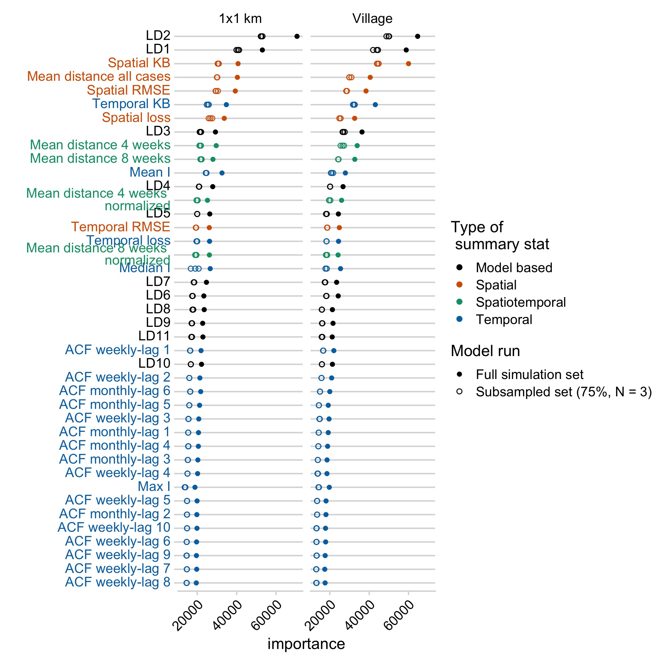
Figure 5.8: Variable importance plots for models run with the full simulation data set (N = 1e5 simulations per model), or subsampled datasets (approx. 75% of the full simulation data set).

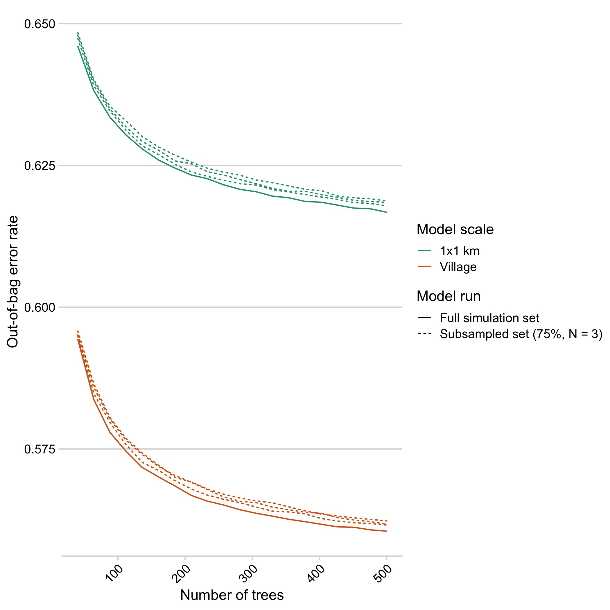
Figure 5.9: Out-of-bag predictions of the out-of-bag error rate as trees are added separated by the scale of the model comparison.

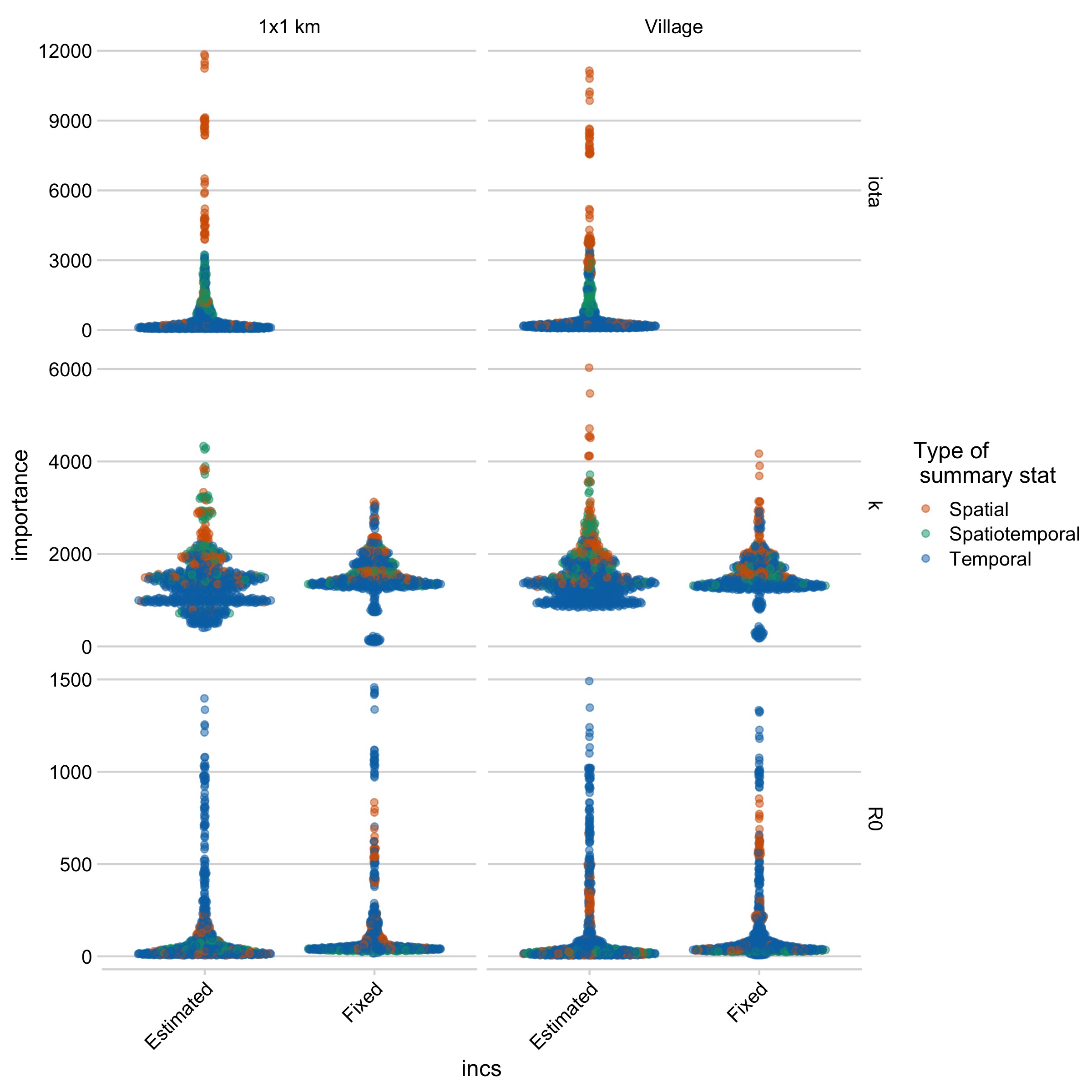
Figure 5.10: Variable importance plots for models run with the full simulation data set (N = 1e5 simulations per model), or subsampled datasets (approx. 75% of the full simulation data set) for each parameter and model.

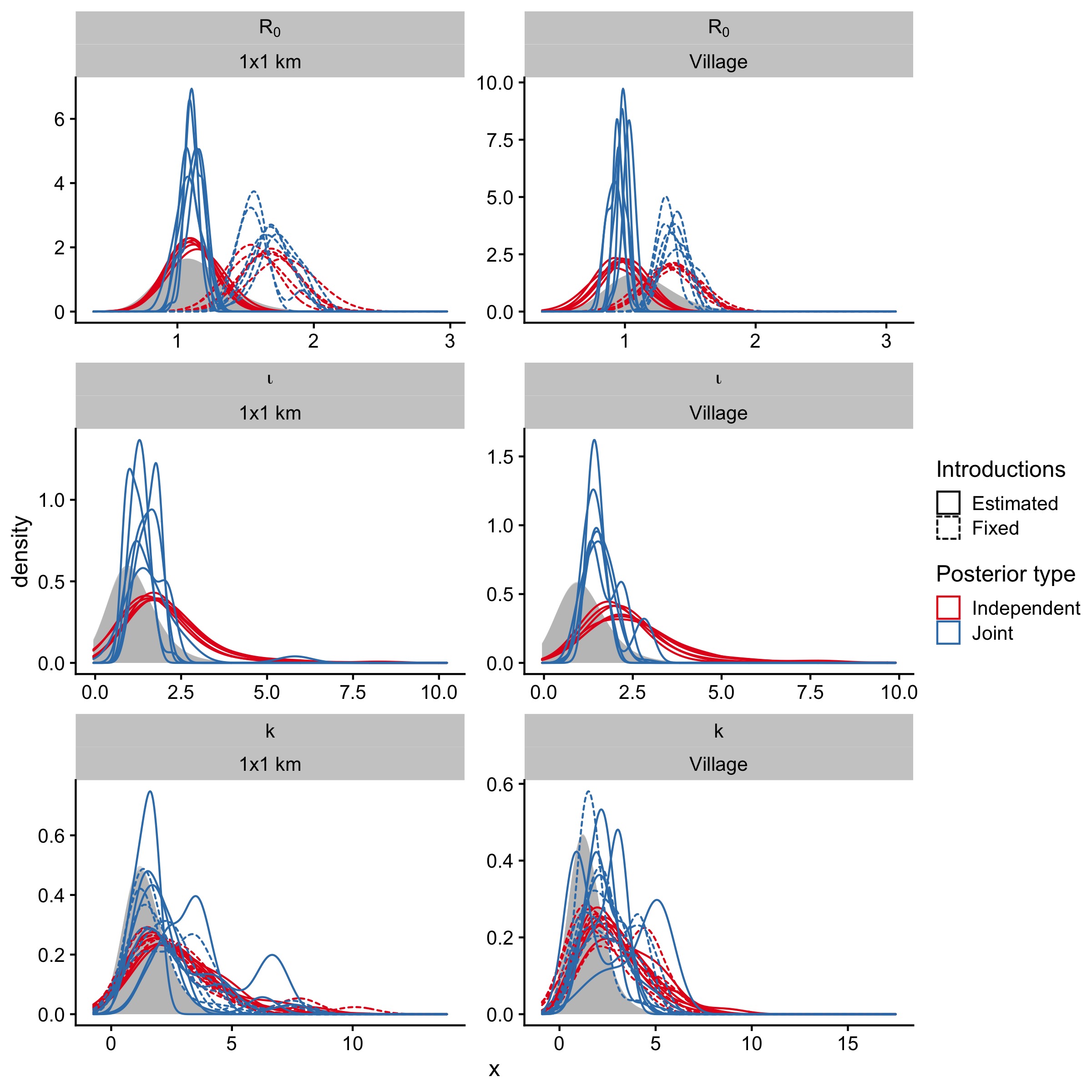
Figure 5.11: Independent posterior estimates for models run with the full simulation data set (N = 1e5 simulations per model), or subsampled datasets (approx. 75% of the full simulation data set) for each parameter and model

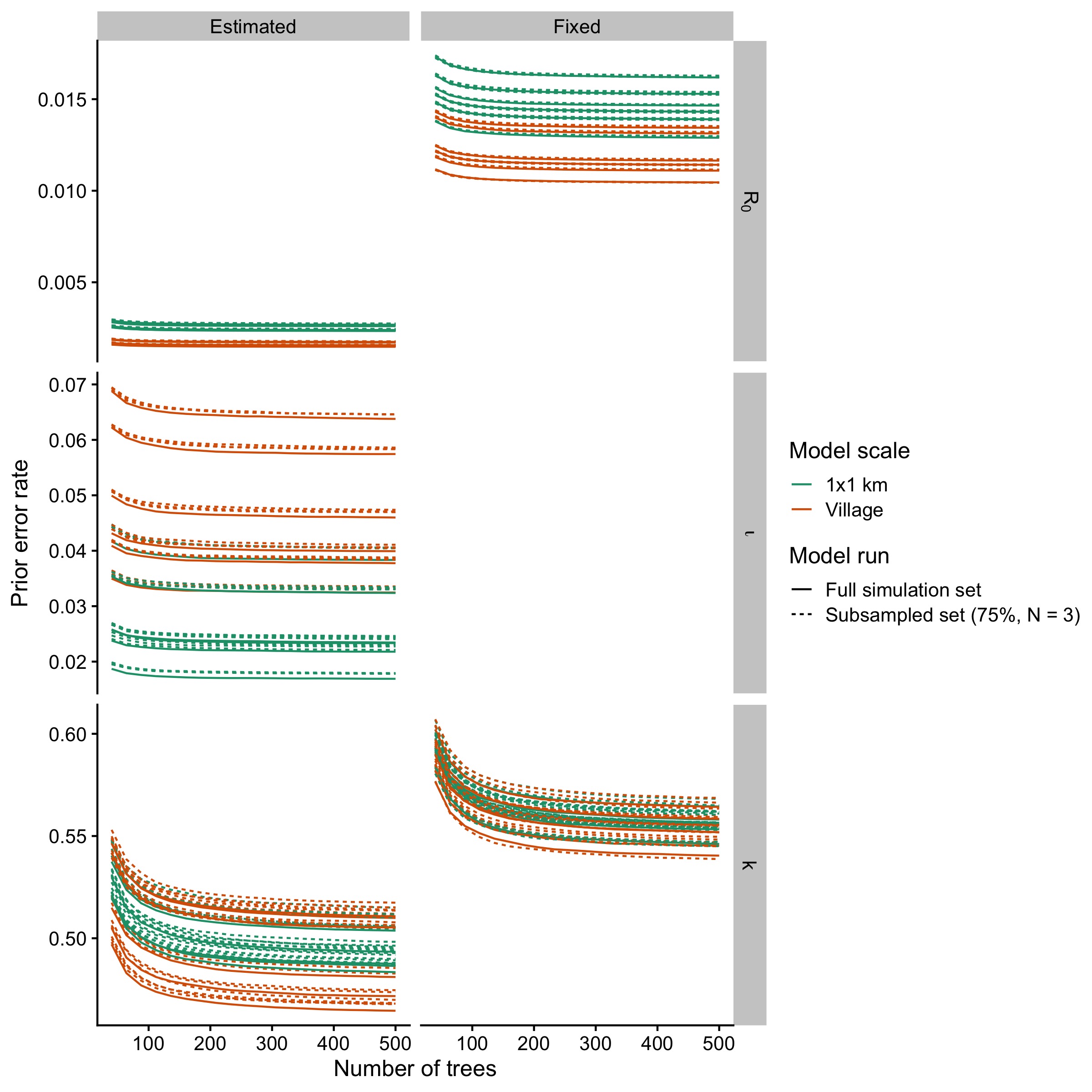
Figure 5.12: Out-of-bag error rates as trees are added separated by the scale of the model comparison and the parameter being estimated.

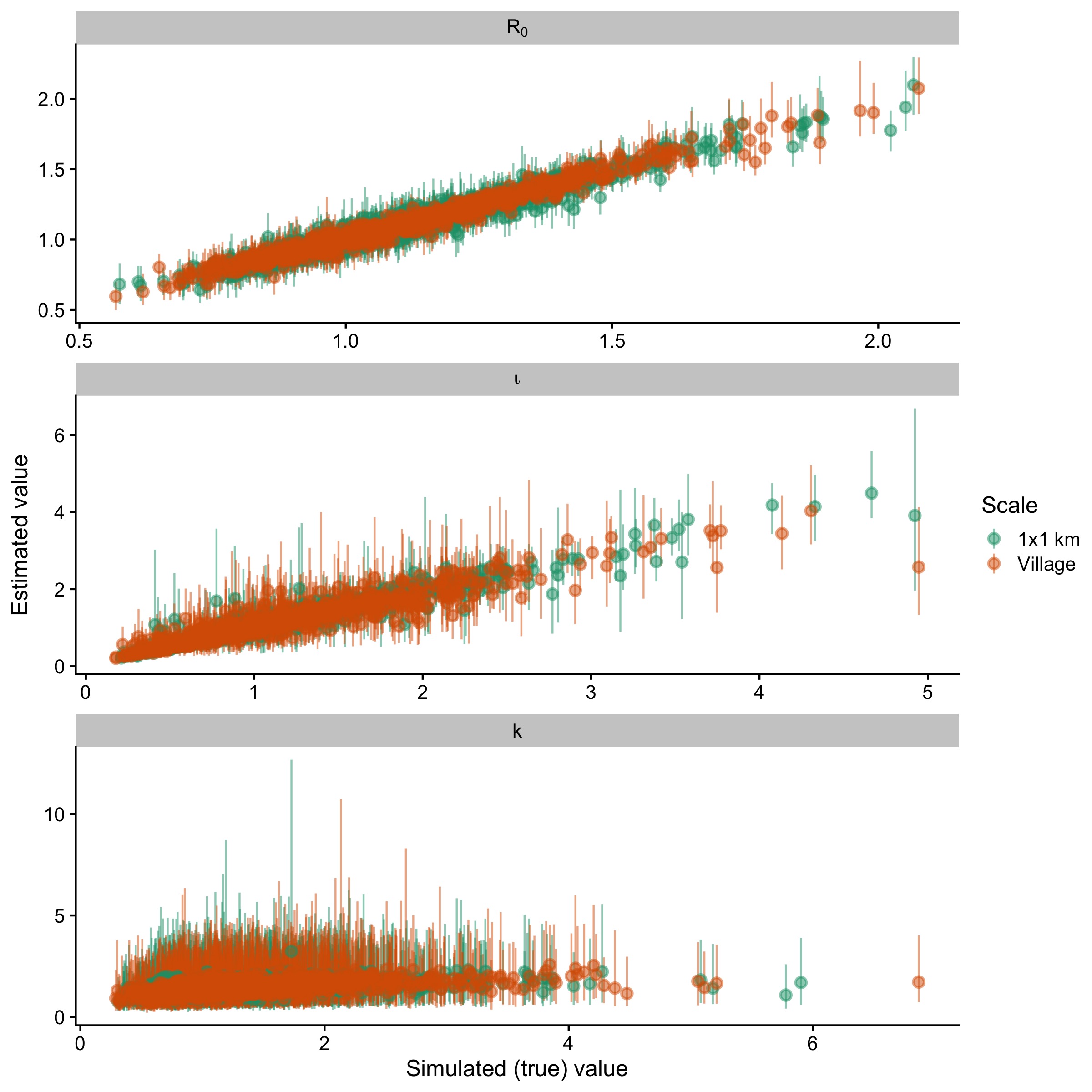
Figure 5.13: Simulated (true) parameter values vs. model estimates for 1000 simulated datasets witheld from the classification model.

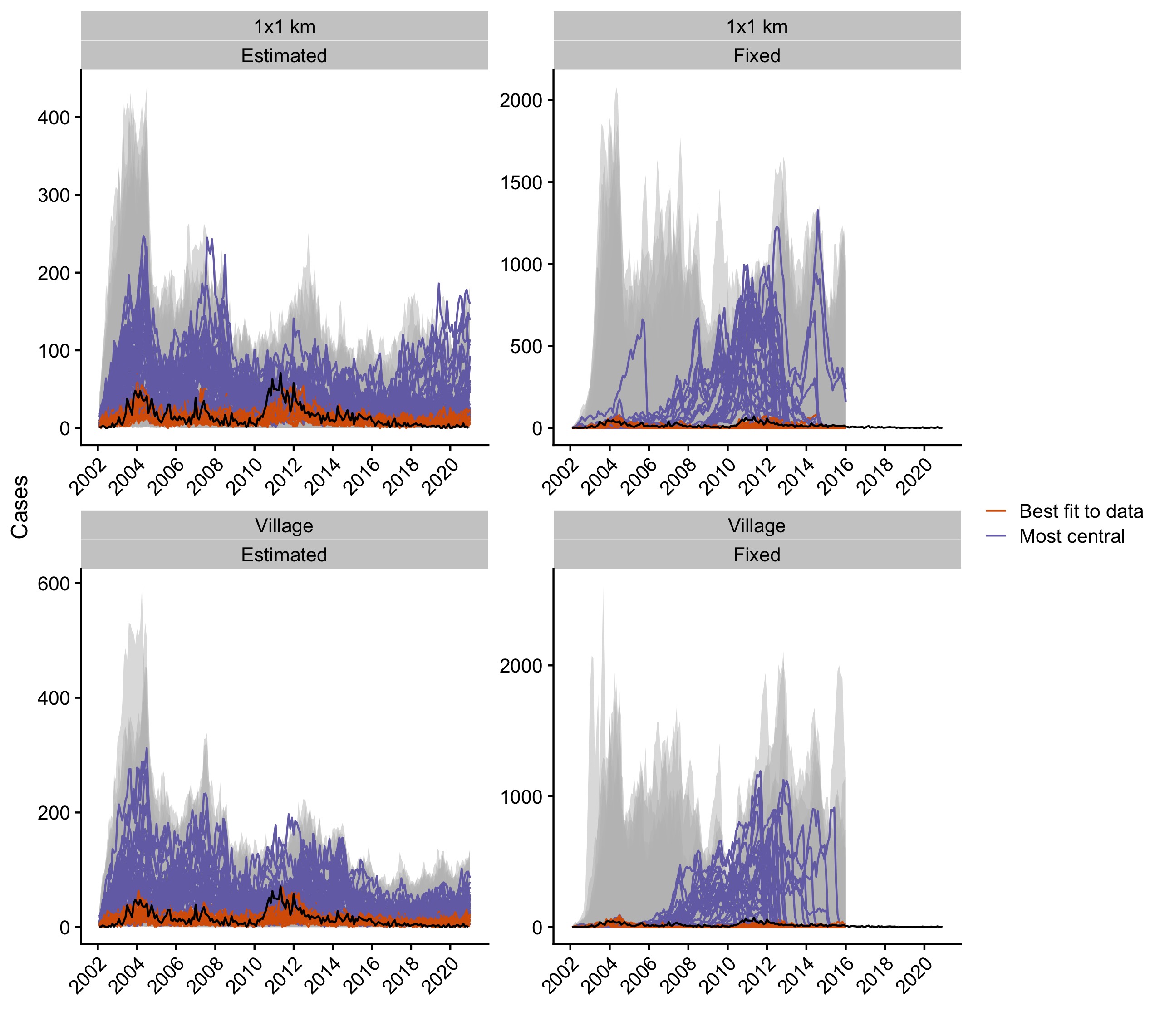
Figure 5.14: Simulations from the independent posterior estimates for all the models. The grey envelope shows the range of simulations, and the black line is the time series of observed monthly cases. The orange lines show the top five simulations that best fit the data (lowest RMSE) and the purple lines show the top five simulations that have the highest centrality score.

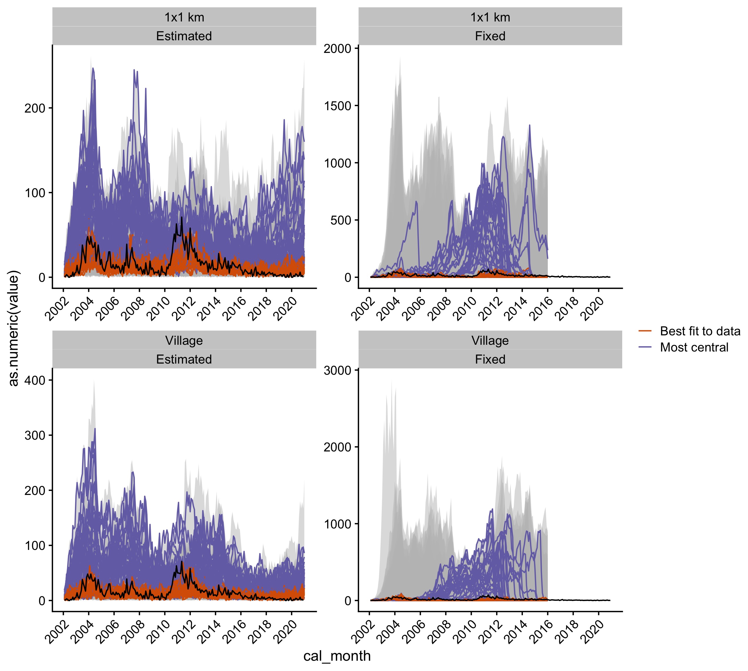
Figure 5.15: Simulations from the joint posterior estimates for all the models. The grey envelope shows the range of simulations, and the black line is the time series of observed monthly cases. The orange lines show the top five simulations that best fit the data (lowest RMSE) and the purple lines show the top five simulations that have the highest centrality score.

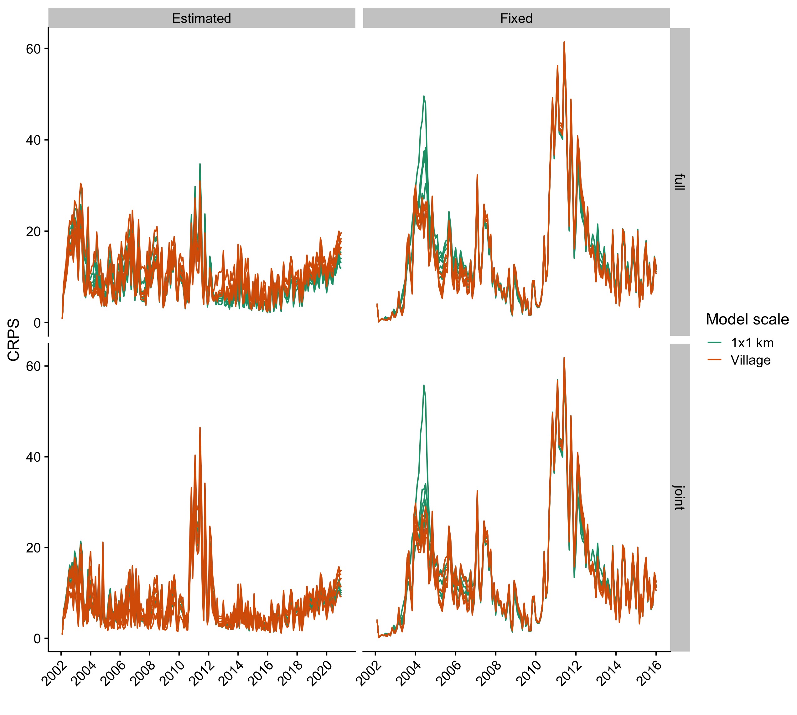
Figure 5.16: Continuous ranked probability scores for the simulated datasets compared to the observed comparing models with estimated introduction rates (columns) and across scales (rows).

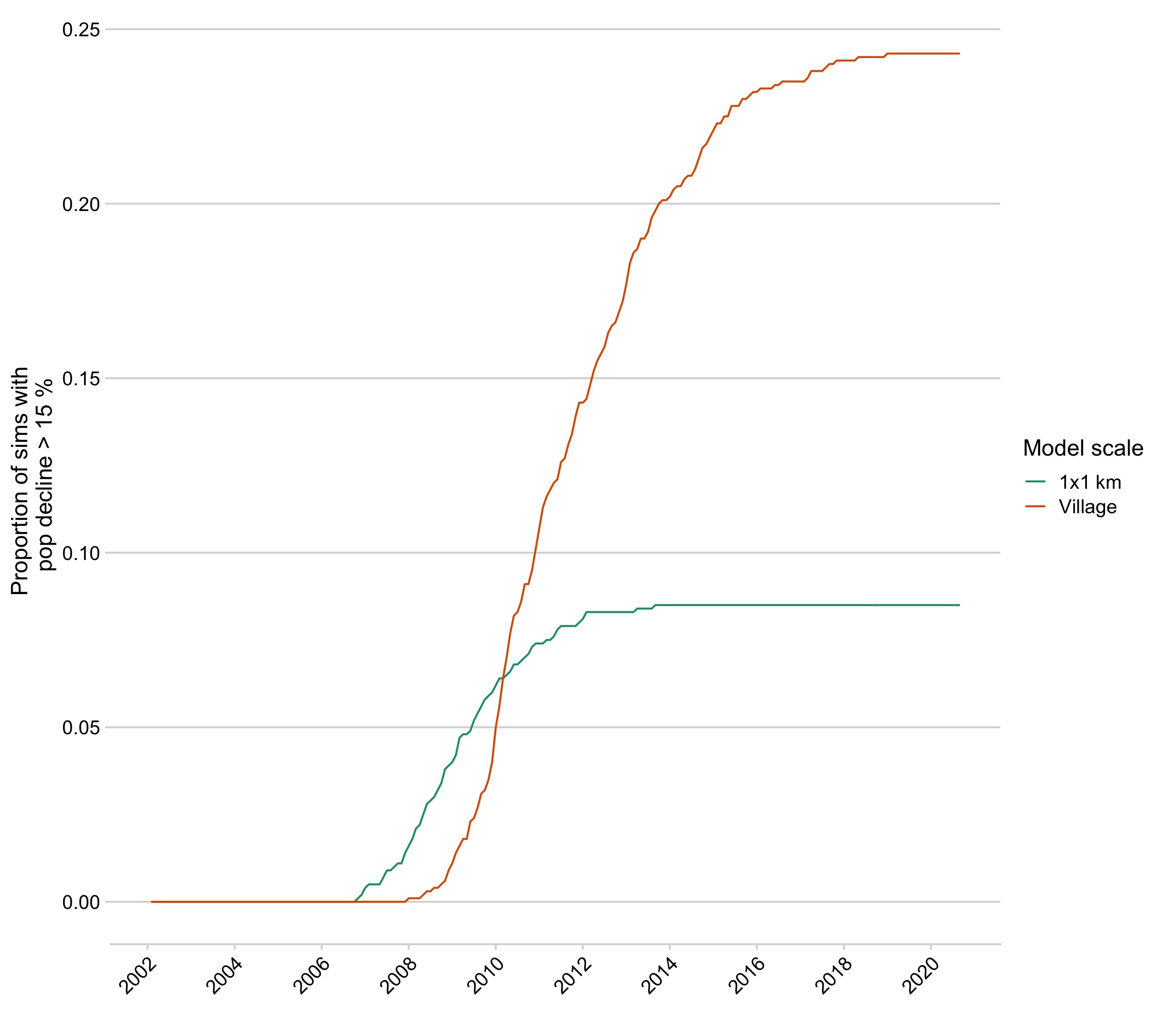
Figure 5.17: The proportion of simulations resulting in population declines > 15% by each time step for the best model at each scale.

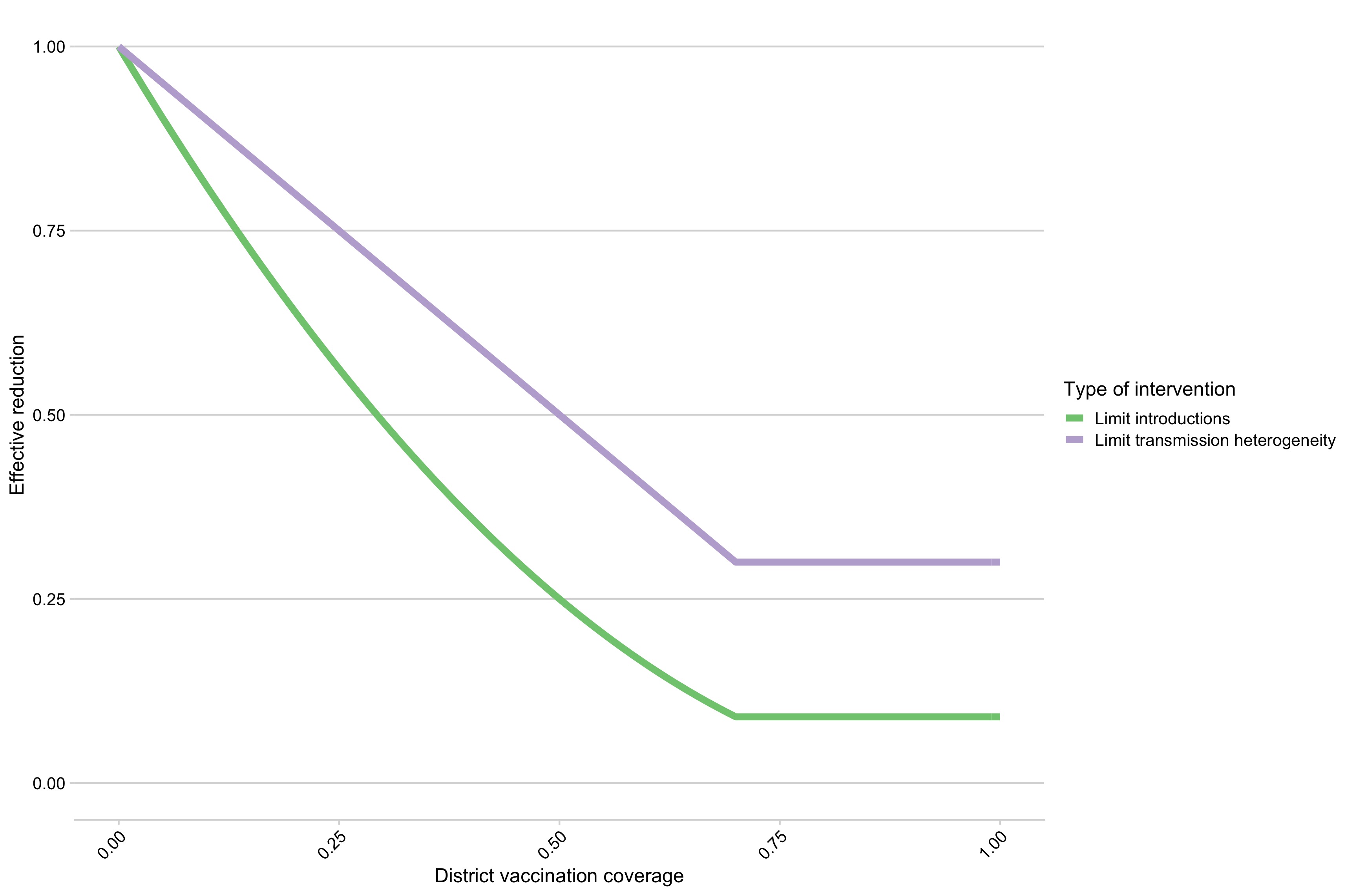
Figure 5.18: The relationship between district level proportion susceptible and reduction in introduction rate and limits on secondary cases.

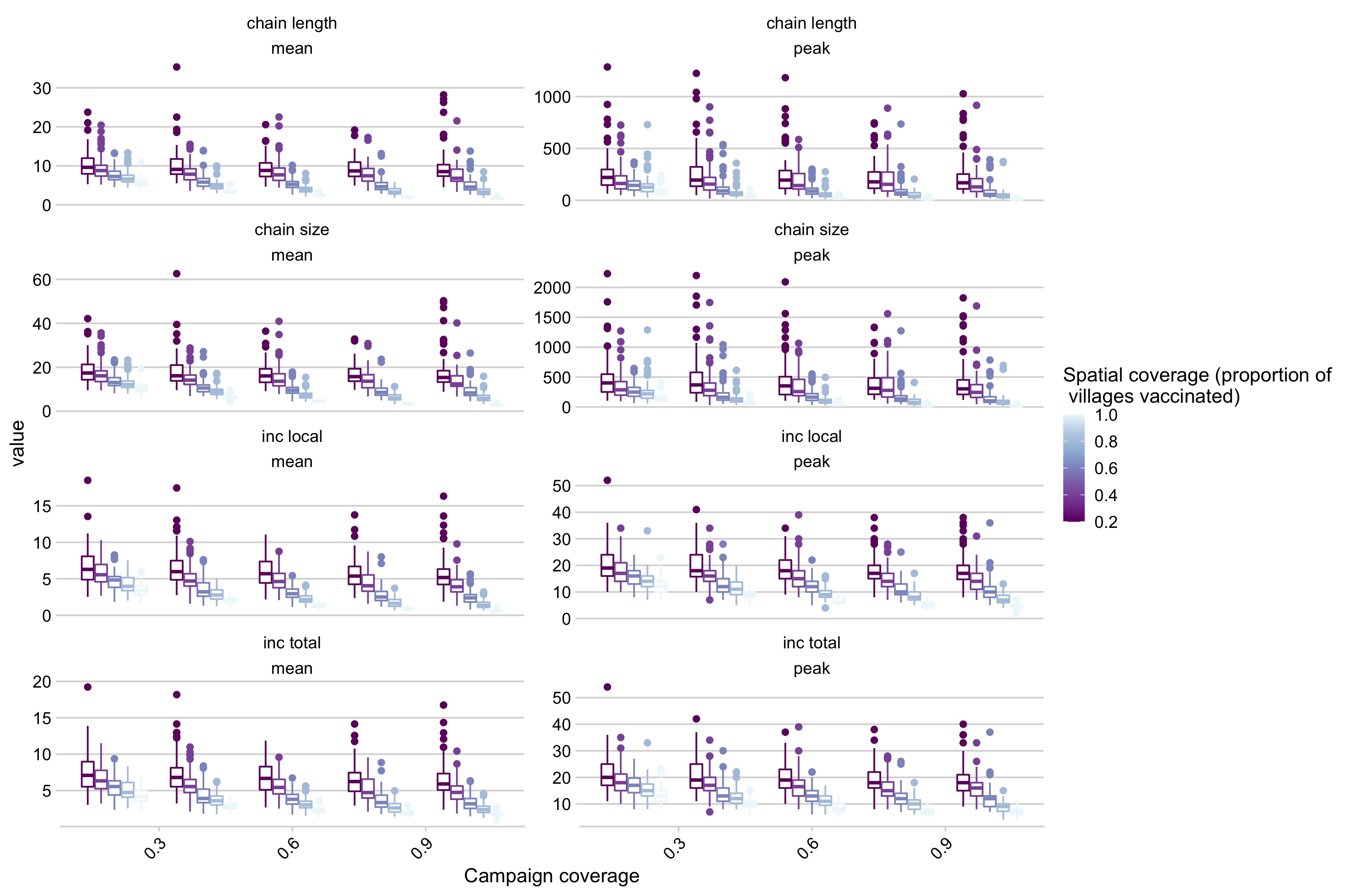
Figure 5.19: Simulation outcomes across a range of campaign coverage and spatial coverage for the baseline case where panels are different summary statistics of the simulations (i.e. chain length mean, chain length peak, etc.).

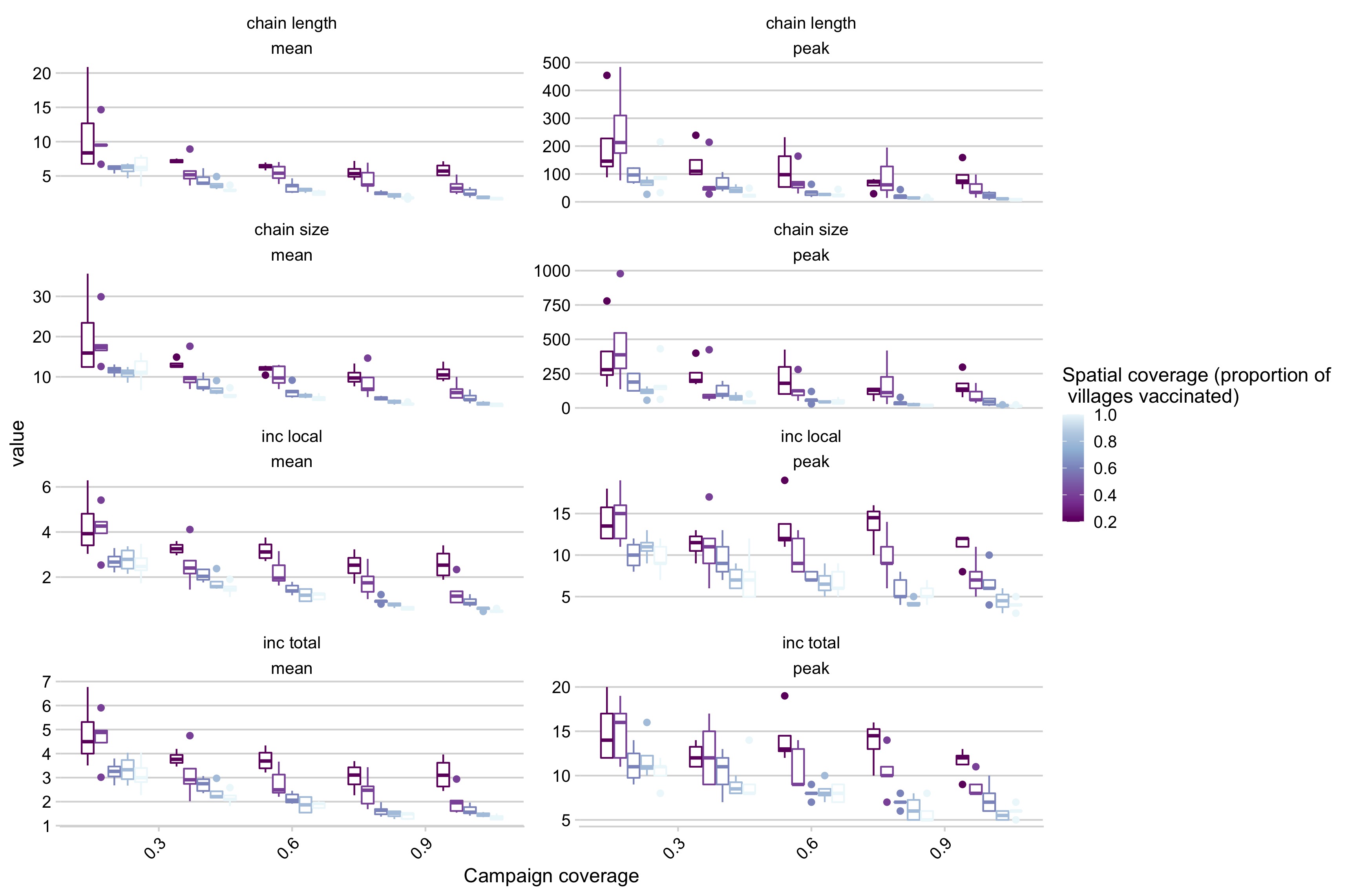
Figure 5.20: Simulation outcomes across a range of campaign coverage and spatial coverage incorporating reductions in the maximum number of secondary cases rate as district coverage increases where panels are different summary statistics of the simulations (i.e. chain length mean, chain length peak, etc.).

Figure 5.21: Simulation outcomes across a range of campaign coverage and spatial coverage incorporating reductions in the introduction rate as district coverage increases where panels are different summary statistics of the simulations (i.e. chain length mean, chain length peak, etc.).

Figure 5.22: Outbreak durations (weeks with cases > 95th % of introductions) and their relationship to connectivity of villages across a range of campaign coverages (i.e. proportion vaccinated in each village, x-axis) and spatial coverage (proportion of villages vaccinated, panels).